 Tweet
Tweet
As a collaboration project with a colleague I did a sequence capture/sequencing experiment. The goal was to sequence the HLA region of a particular haplotype associated with a particular disease. My Agilent rep gave me early access to a SureSelect HLA capture product that seemed to work pretty well. I got a library that sequenced well, and an initial alignment with the HLA region yielded decent coverage and on-target numbers. Now, however, I'm trying to do more analysis of it and need some help.
I'm well-versed in the bench-work of this type, but I'm still a novice when it comes to genomic data analysis. For the initial alignment I mentioned, I just mapped the reads to a FASTA file of the HLA region using Roche's Assembler software. That's not annotated or anything, though, so it's not very useful. I have a .bed file describing the baits, and I've used that at the UCSC Genome Browser site to visualize them, and found that the captured region covers a little more than what was in the FASTA used for the initial alignment, and that there are some fairly large gaps that aren't covered by the baits. Is there a way I can use the .bed file to download a better reference file that covers just the captured region and not the gaps?
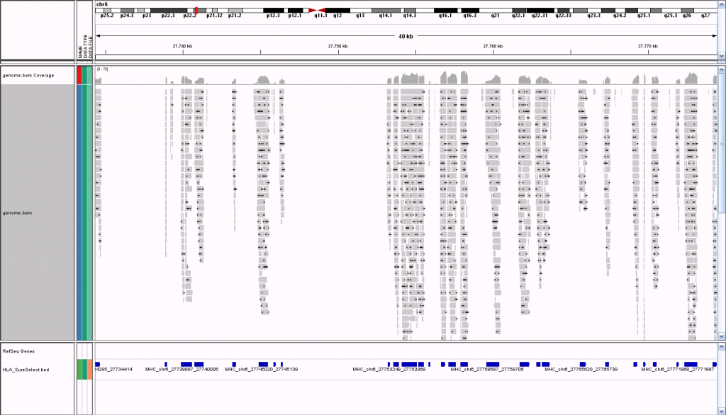
Also, I loaded the BAM file from that alignment into GenomeBrowse to visualize the the data but that didn't work at all. I can't say I'm surprised, though, because it was only aligned to a FASTA file with a few Mb of data, not the whole genome. What is the right way to go about visualizing the data?
I'm well-versed in the bench-work of this type, but I'm still a novice when it comes to genomic data analysis. For the initial alignment I mentioned, I just mapped the reads to a FASTA file of the HLA region using Roche's Assembler software. That's not annotated or anything, though, so it's not very useful. I have a .bed file describing the baits, and I've used that at the UCSC Genome Browser site to visualize them, and found that the captured region covers a little more than what was in the FASTA used for the initial alignment, and that there are some fairly large gaps that aren't covered by the baits. Is there a way I can use the .bed file to download a better reference file that covers just the captured region and not the gaps?
Also, I loaded the BAM file from that alignment into GenomeBrowse to visualize the the data but that didn't work at all. I can't say I'm surprised, though, because it was only aligned to a FASTA file with a few Mb of data, not the whole genome. What is the right way to go about visualizing the data?

Comment